2D Biased Double Well

Estimation of an overdamped Langevin in presence of biased dynamics.

import numpy as np
import matplotlib.pyplot as plt
import folie as fl
from mpl_toolkits.mplot3d import Axes3D
from copy import deepcopy
import time

checkpoint1 = time.time()
x = np.linspace(-1.8, 1.8, 36)
y = np.linspace(-1.8, 1.8, 36)
input = np.transpose(np.array([x, y]))

D = 0.5
diff_function = fl.functions.Polynomial(deg=0, coefficients=D * np.eye(2, 2))
a, b = 5, 10
drift_quartic2d = fl.functions.Quartic2D(a=D * a, b=D * b)  # simple way to multiply D*Potential here force is the SDE force (meandispl)  ## use this when you need the drift ###
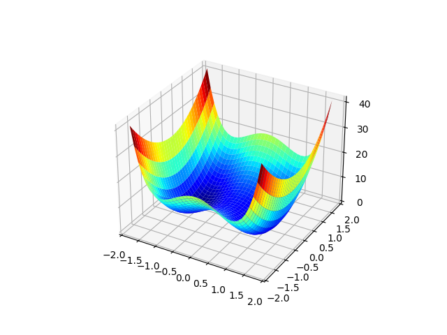
quartic2d = fl.functions.Quartic2D(a=a, b=b)  # Real potential , here force is just -grad pot ## use this when you need the potential energy ###

X, Y = np.meshgrid(x, y)

# Plot potential surface
pot = quartic2d.potential_plot(X, Y)
fig = plt.figure()
ax = plt.axes(projection="3d")
ax.plot_surface(X, Y, pot, rstride=1, cstride=1, cmap="jet", edgecolor="none")

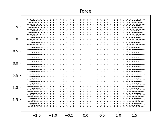
# Plot Force function
ff = quartic2d.force(input)  # returns x and y components of the force : x_comp =ff[:,0] , y_comp =ff[:,1]
U, V = np.meshgrid(ff[:, 0], ff[:, 1])
fig, ax = plt.subplots()
ax.quiver(x, y, U, V)
ax.set_title("Force")


##Definition of the Collective variable function of old coordinates
def colvar(x, y):
    gradient = np.array([1, 1])
    return x + y, gradient  # need to return both colvar function q=q(x,y) and gradient (dq/dx,dq/dy)


dt = 1e-3
model_simu = fl.models.overdamped.Overdamped(drift_quartic2d, diffusion=diff_function)
simulator = fl.simulations.ABMD_2D_to_1DColvar_Simulator(fl.simulations.EulerStepper(model_simu), dt, colvar=colvar, k=25.0, qstop=1.2)

# Choose number of trajectories and initialize positions
ntraj = 20
q0 = np.empty(shape=[ntraj, 2])
for i in range(ntraj):
    for j in range(2):
        q0[i][j] = -1.2

• 
• 

# CALCULATE TRAJECTORY ##

time_steps = 10000
data = simulator.run(time_steps, q0, save_every=1)

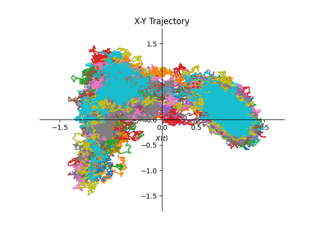
# Plot the resulting trajectories
fig, axs = plt.subplots()
for n, trj in enumerate(data):
    axs.plot(trj["x"][:, 0], trj["x"][:, 1])
    axs.spines["left"].set_position("center")
    axs.spines["right"].set_color("none")
    axs.spines["bottom"].set_position("center")
    axs.spines["top"].set_color("none")
    axs.xaxis.set_ticks_position("bottom")
    axs.yaxis.set_ticks_position("left")
    axs.set_xlabel("$X(t)$")
    axs.set_ylabel("$Y(t)$")
    axs.set_title("X-Y Trajectory")
    axs.set_xlim(-1.8, 1.8)
    axs.set_ylim(-1.8, 1.8)
    axs.grid()

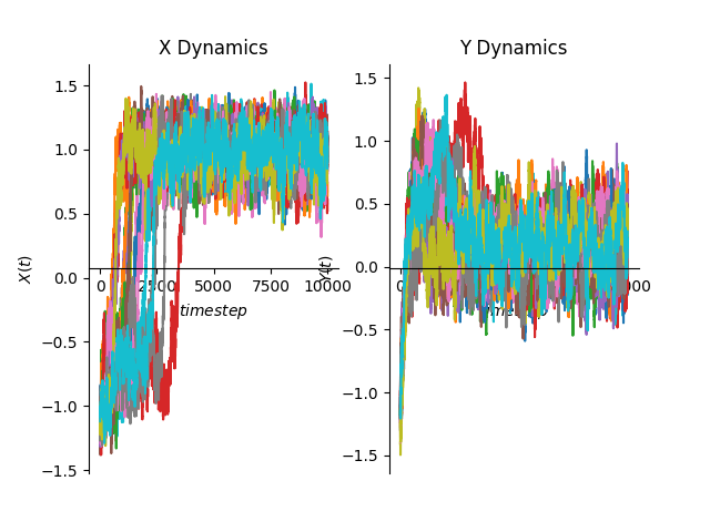
# plot x,y Trajectories in separate subplots
fig, bb = plt.subplots(1, 2)
for n, trj in enumerate(data):
    bb[0].plot(trj["x"][:, 0])
    bb[1].plot(trj["x"][:, 1])

    # Set visible  axis
    bb[0].spines["right"].set_color("none")
    bb[0].spines["bottom"].set_position("center")
    bb[0].spines["top"].set_color("none")
    bb[0].xaxis.set_ticks_position("bottom")
    bb[0].yaxis.set_ticks_position("left")
    bb[0].set_xlabel("$timestep$")
    bb[0].set_ylabel("$X(t)$")

    # Set visible axis
    bb[1].spines["right"].set_color("none")
    bb[1].spines["bottom"].set_position("center")
    bb[1].spines["top"].set_color("none")
    bb[1].xaxis.set_ticks_position("bottom")
    bb[1].yaxis.set_ticks_position("left")
    bb[1].set_xlabel("$timestep$")
    bb[1].set_ylabel("$Y(t)$")

    bb[0].set_title("X Dynamics")
    bb[1].set_title("Y Dynamics")

• 
• 

PROJECTION ALONG CHOSEN COORDINATE #

# Choose unit versor of direction
u = np.array([1, 1])
u_norm = (1 / np.linalg.norm(u, 2)) * u
w = np.empty_like(trj["x"][:, 0])
b = np.empty_like(trj["x"][:, 0])
proj_data = fl.data.trajectories.Trajectories(dt=dt)  # create new Trajectory object in which to store the projected trajectory dictionaries
fig, axs = plt.subplots()
for n, trj in enumerate(data):
    for i in range(len(trj["x"])):
        w[i] = np.dot(trj["x"][i], u_norm)
        b[i] = np.dot(trj["bias"][i], u_norm)
    proj_data.append(fl.Trajectory(1e-3, deepcopy(w.reshape(len(trj["x"][:, 0]), 1)), bias=deepcopy(b.reshape(len(trj["bias"][:, 0]), 1))))
    axs.plot(proj_data[n]["x"])
    axs.set_xlabel("$timesteps$")
    axs.set_ylabel("$w(t)$")
    axs.set_title("trajectory projected along $u =$" + str(u) + " direction")
    axs.grid()

# MODEL TRAINING ##

checkpoint2 = time.time()

domain = fl.MeshedDomain.create_from_range(np.linspace(proj_data.stats.min, proj_data.stats.max, 4).ravel())
trainmodel = fl.models.OverdampedSplines1D(domain=domain)

xfa = np.linspace(proj_data.stats.min, proj_data.stats.max, 75)
drift_exact = (xfa**2 - 1.0) ** 2

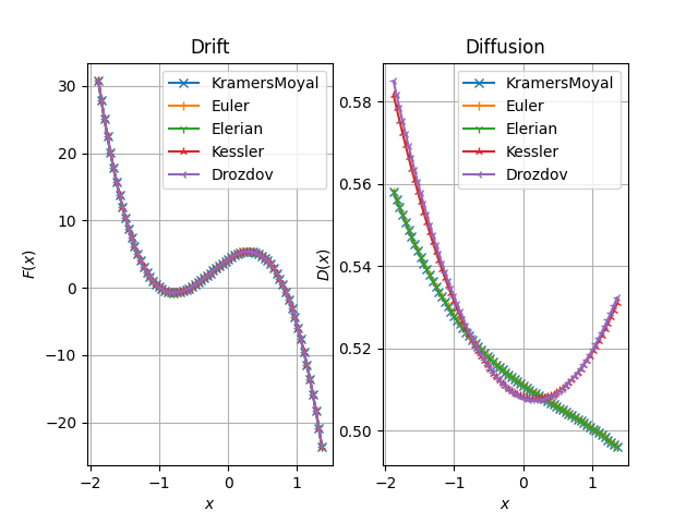
fig, axs = plt.subplots(1, 2)
axs[0].set_title("Drift")
axs[0].set_xlabel("$x$")
axs[0].set_ylabel("$F(x)$")
axs[0].grid()
axs[1].set_title("Diffusion")
axs[1].set_xlabel("$x$")
axs[1].set_ylabel("$D(x)$")
axs[1].grid()


KM_Estimator = fl.KramersMoyalEstimator(deepcopy(trainmodel))
res_KM = KM_Estimator.fit_fetch(proj_data)

axs[0].plot(xfa, res_KM.drift(xfa.reshape(-1, 1)), marker="x", label="KramersMoyal")
axs[1].plot(xfa, res_KM.diffusion(xfa.reshape(-1, 1)), marker="x", label="KramersMoyal")
print("KramersMoyal ", res_KM.coefficients)
for name, marker, transitioncls in zip(
    ["Euler", "Elerian", "Kessler", "Drozdov"],
    ["|", "1", "2", "3"],
    [
        fl.EulerDensity,
        fl.ElerianDensity,
        fl.KesslerDensity,
        fl.DrozdovDensity,
    ],
):
    estimator = fl.LikelihoodEstimator(transitioncls(deepcopy(trainmodel)))
    res = estimator.fit_fetch(deepcopy(proj_data))
    print(name, res.coefficients)
    axs[0].plot(xfa, res.drift(xfa.reshape(-1, 1)), marker=marker, label=name)
    axs[1].plot(xfa, res.diffusion(xfa.reshape(-1, 1)), marker=marker, label=name)

axs[0].legend()
axs[1].legend()
checkpoint3 = time.time()

print("Training time =", checkpoint3 - checkpoint2, "seconds")
print("Overall time =", checkpoint3 - checkpoint1, "seconds")

plt.show()

KramersMoyal  [ 30.71649137 -43.67528562  47.17982055 -23.67474057   0.55823587
   0.50837918   0.51151879   0.49603091]
Euler [ 30.71649137 -43.67528562  47.17982055 -23.67474057   0.55823587
   0.50837918   0.51151879   0.49603091]
Elerian [ 30.71649137 -43.67528562  47.17982055 -23.67474057   0.55823587
   0.50837918   0.51151879   0.49603091]
Kessler [ 30.71676539 -43.67519393  47.17997269 -23.67517801   0.58169736
   0.50211745   0.48933294   0.53096499]
Drozdov [ 30.71670615 -43.67521385  47.17999026 -23.67509516   0.58501043
   0.50211185   0.48743717   0.53233277]
Training time = 11.307701826095581 seconds
Overall time = 14.38679313659668 seconds