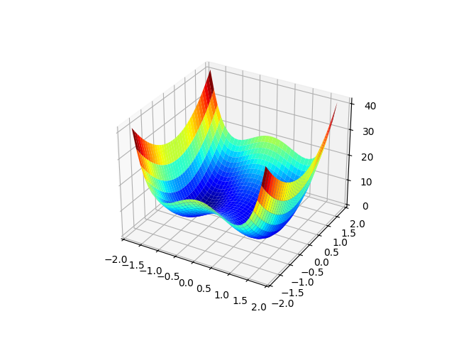
2D Double Well

Estimation of an overdamped Langevin.

import numpy as np
import matplotlib.pyplot as plt
import folie as fl
from mpl_toolkits.mplot3d import Axes3D
from copy import deepcopy

""" Script for simulation of 2D double well and projection along user provided direction, No fitting is carried out   """
x = np.linspace(-1.8, 1.8, 36)
y = np.linspace(-1.8, 1.8, 36)
input = np.transpose(np.array([x, y]))

D = 0.5
diff_function = fl.functions.Polynomial(deg=0, coefficients=D * np.eye(2, 2))
a, b = 5, 10
drift_quartic2d = fl.functions.Quartic2D(a=D * a, b=D * b)  # simple way to multiply D*Potential here force is the SDE force (meandispl)  ## use this when you need the drift ###
quartic2d = fl.functions.Quartic2D(a=a, b=b)  # Real potential , here force is just -grad pot ## use this when you need the potential energy ###

X, Y = np.meshgrid(x, y)

# Plot potential surface
pot = quartic2d.potential_plot(X, Y)

fig = plt.figure()
ax = plt.axes(projection="3d")
ax.plot_surface(X, Y, pot, rstride=1, cstride=1, cmap="jet", edgecolor="none")

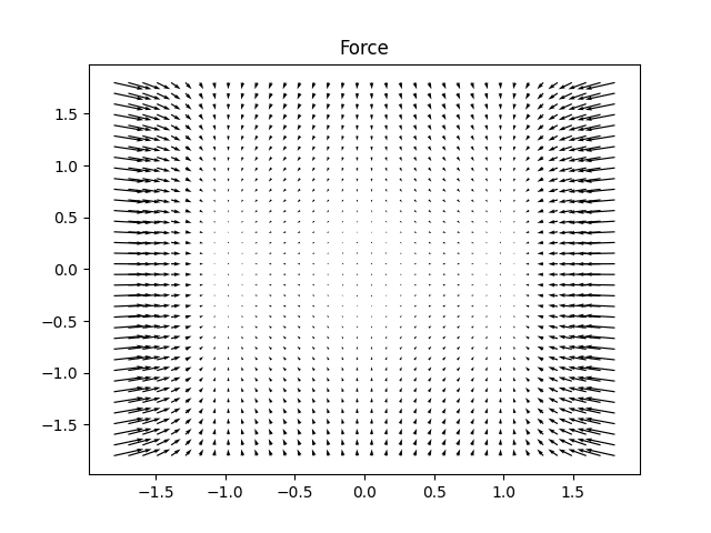
# Plot Force function
ff = quartic2d.force(input)  # returns x and y components of the force : x_comp =ff[:,0] , y_comp =ff[:,1]
U, V = np.meshgrid(ff[:, 0], ff[:, 1])
fig, ax = plt.subplots()
ax.quiver(x, y, U, V)
ax.set_title("Force")

dt = 5e-4
model_simu = fl.models.overdamped.Overdamped(drift_quartic2d, diffusion=diff_function)
simulator = fl.simulations.Simulator(fl.simulations.EulerStepper(model_simu), dt)

# initialize positions
ntraj = 30
q0 = np.empty(shape=[ntraj, 2])
for i in range(ntraj):
    for j in range(2):
        q0[i][j] = 0.000

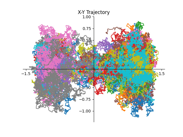
# Calculate Trajectory
time_steps = 3000
data = simulator.run(time_steps, q0, save_every=1)

# Plot the resulting trajectories
fig, axs = plt.subplots()
for n, trj in enumerate(data):
    axs.plot(trj["x"][:, 0], trj["x"][:, 1])
    axs.spines["left"].set_position("center")
    axs.spines["right"].set_color("none")
    axs.spines["bottom"].set_position("center")
    axs.spines["top"].set_color("none")
    axs.xaxis.set_ticks_position("bottom")
    axs.yaxis.set_ticks_position("left")
    axs.set_xlabel("$X(t)$")
    axs.set_ylabel("$Y(t)$")
    axs.set_title("X-Y Trajectory")
    axs.grid()

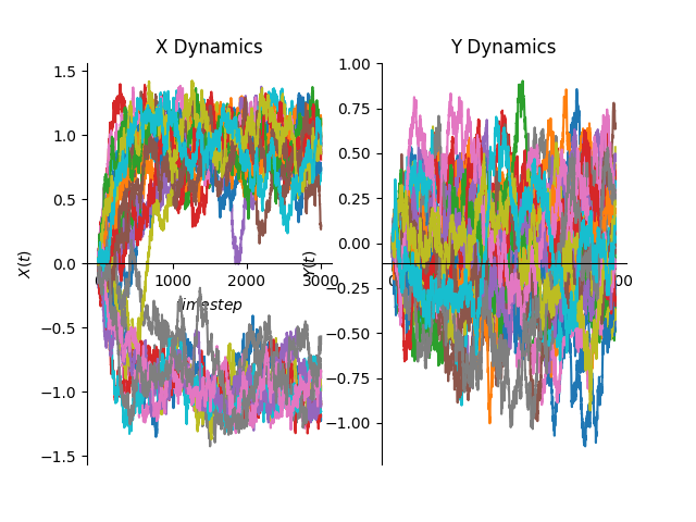
# plot Trajectories
fig, bb = plt.subplots(1, 2)
for n, trj in enumerate(data):
    bb[0].plot(trj["x"][:, 0])
    bb[1].plot(trj["x"][:, 1])

    # Set visible  axis
    bb[0].spines["right"].set_color("none")
    bb[0].spines["bottom"].set_position("center")
    bb[0].spines["top"].set_color("none")
    bb[0].xaxis.set_ticks_position("bottom")
    bb[0].yaxis.set_ticks_position("left")
    bb[0].set_xlabel("$timestep$")
    bb[0].set_ylabel("$X(t)$")

    # Set visible axis
    bb[1].spines["right"].set_color("none")
    bb[1].spines["bottom"].set_position("center")
    bb[1].spines["top"].set_color("none")
    bb[1].xaxis.set_ticks_position("bottom")
    bb[1].yaxis.set_ticks_position("left")
    bb[1].set_xlabel("$timestep$")
    bb[1].set_ylabel("$Y(t)$")

    bb[0].set_title("X Dynamics")
    bb[1].set_title("Y Dynamics")

• 
• 
• 
• 

PROJECTION ALONG CHOSEN COORDINATE #

# Choose unit versor of direction
u = np.array([1, 1])
u_norm = (1 / np.linalg.norm(u, 2)) * u
w = np.empty_like(trj["x"][:, 0])
proj_data = fl.Trajectories(dt=1e-3)
fig, axs = plt.subplots()
for n, trj in enumerate(data):
    for i in range(len(trj["x"])):
        w[i] = np.dot(trj["x"][i], u_norm)
    proj_data.append(fl.Trajectory(1e-3, deepcopy(w.reshape(len(trj["x"][:, 0]), 1))))
    axs.plot(proj_data[n]["x"])
    axs.set_xlabel("$timesteps$")
    axs.set_ylabel("$w(t)$")
    axs.set_title("trajectory projected along $u =$" + str(u) + " direction")
    axs.grid()

plt.show()