1D Biased Double Well

Estimation of an overdamped Langevin in presence of biased dynamics.

• 
• 
• 

Euler [  4.22054548 -12.51555831  13.83274923  -6.30298083   0.48478253
   0.52170744   0.49355682   0.5007274 ]
Elerian [  4.22054795 -12.51555549  13.83275452  -6.30296867   0.48487525
   0.52178501   0.49358168   0.50077429]
Kessler [  4.22055274 -12.51553497  13.83277905  -6.30292702   0.48667153
   0.52063655   0.4921984    0.50298026]
Drozdov [  4.22057785 -12.5155274   13.83278778  -6.3029196    0.48686415
   0.52065394   0.49209304   0.50305591]

import numpy as np
import matplotlib.pyplot as plt
import folie as fl
from copy import deepcopy

coeff = 0.2 * np.array([0, 0, -4.5, 0, 0.1])
free_energy = np.polynomial.Polynomial(coeff)
D = np.array([0.5])

drift_coeff = D * np.array([-coeff[1], -2 * coeff[2], -3 * coeff[3], -4 * coeff[4]])
drift_function = fl.functions.Polynomial(deg=3, coefficients=drift_coeff)
diff_function = fl.functions.Polynomial(deg=0, coefficients=D)

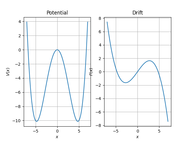
# Plot of Free Energy and Force
x_values = np.linspace(-7, 7, 100)
fig, axs = plt.subplots(1, 2)
axs[0].plot(x_values, free_energy(x_values))
axs[1].plot(x_values, drift_function(x_values.reshape(len(x_values), 1)))
axs[0].set_title("Potential")
axs[0].set_xlabel("$x$")
axs[0].set_ylabel("$V(x)$")
axs[0].grid()
axs[1].set_title("Drift")
axs[1].set_xlabel("$x$")
axs[1].set_ylabel("$F(x)$")
axs[1].grid()

# Define model to simulate and type of simulator to use
model_simu = fl.models.overdamped.Overdamped(drift_function, diffusion=diff_function)
simulator = fl.simulations.ABMD_Simulator(fl.simulations.EulerStepper(model_simu), 1e-3, k=10.0, xstop=6.0)

# initialize positions
ntraj = 30
q0 = np.empty(ntraj)
for i in range(len(q0)):
    q0[i] = -6
# Calculate Trajectory
time_steps = 25000
data = simulator.run(time_steps, q0, save_every=1)
xmax = np.concatenate(simulator.xmax_hist, axis=1).T

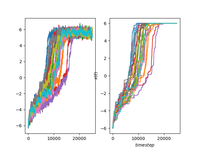
# Plot the resulting trajectories
fig, axs = plt.subplots(1, 2)
for n, trj in enumerate(data):
    axs[0].plot(trj["x"])
    axs[1].plot(xmax[:, n])
    axs[1].set_xlabel("$timestep$")
    axs[1].set_ylabel("$x(t)$")
    axs[1].grid()

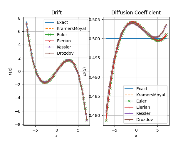
fig, axs = plt.subplots(1, 2)
axs[0].set_title("Drift")
axs[0].set_xlabel("$x$")
axs[0].set_ylabel("$F(x)$")
axs[0].grid()

axs[1].set_title("Diffusion Coefficient")  # i think should be diffusion coefficient
axs[1].set_xlabel("$x$")
axs[1].set_ylabel("$D(x)$")
axs[1].grid()

xfa = np.linspace(-7.0, 7.0, 75)
model_simu.remove_bias()
axs[0].plot(xfa, model_simu.drift(xfa.reshape(-1, 1)), label="Exact")
axs[1].plot(xfa, model_simu.diffusion(xfa.reshape(-1, 1)), label="Exact")

domain = fl.MeshedDomain.create_from_range(np.linspace(data.stats.min, data.stats.max, 4).ravel())
trainmodel = fl.models.Overdamped(fl.functions.BSplinesFunction(domain), has_bias=True)

name = "KramersMoyal"
estimator = fl.KramersMoyalEstimator(trainmodel)
res = estimator.fit_fetch(data)
res.remove_bias()
axs[0].plot(xfa, res.drift(xfa.reshape(-1, 1)), "--", label=name)
axs[1].plot(xfa, res.diffusion(xfa.reshape(-1, 1)), "--", label=name)


for name, marker, transitioncls in zip(
    ["Euler", "Elerian", "Kessler", "Drozdov"],
    ["x", "1", "2", "3"],
    [
        fl.EulerDensity,
        fl.ElerianDensity,
        fl.KesslerDensity,
        fl.DrozdovDensity,
    ],
):
    trainmodel = fl.models.Overdamped(fl.functions.BSplinesFunction(domain), has_bias=True)
    estimator = fl.LikelihoodEstimator(transitioncls(trainmodel), n_jobs=4)

    res = estimator.fit_fetch(deepcopy(data))

    print(name, res.coefficients)
    res.remove_bias()
    axs[0].plot(xfa, res.drift(xfa.reshape(-1, 1)), marker=marker, label=name)
    axs[1].plot(xfa, res.diffusion(xfa.reshape(-1, 1)), marker=marker, label=name)
axs[0].legend()
axs[1].legend()
plt.show()