1D Double Well

Estimation of an overdamped Langevin.

• 
• 
• 

import numpy as np
import matplotlib.pyplot as plt
import folie as fl

coeff = 0.2 * np.array([0, 0, -4.5, 0, 0.1])
free_energy = np.polynomial.Polynomial(coeff)
D = 0.5
drift_coeff = D * np.array([-coeff[1], -2 * coeff[2], -3 * coeff[3], -4 * coeff[4]])

drift_function = fl.functions.Polynomial(deg=3, coefficients=drift_coeff)
diff_function = fl.functions.Polynomial(deg=0, coefficients=np.array(D))

# Plot of Free Energy and Force
x_values = np.linspace(-7, 7, 100)
# fig, axs = plt.subplots(1, 2)
# axs[0].plot(x_values, free_energy(x_values))
# axs[1].plot(x_values, drift_function(x_values.reshape(len(x_values), 1)))
# axs[0].set_title("Potential")
# axs[0].set_xlabel("$x$")
# axs[0].set_ylabel("$V(x)$")
# axs[0].grid()
# axs[1].set_title("Force")
# axs[1].set_xlabel("$x$")
# axs[1].set_ylabel("$F(x)$")
# axs[1].grid()

# Define model to simulate and type of simulator to use
dt = 1e-3
model_simu = fl.models.overdamped.Overdamped(drift_function, diffusion=diff_function)
simulator = fl.simulations.Simulator(fl.simulations.EulerStepper(model_simu), dt)


# initialize positions
ntraj = 30
q0 = np.empty(ntraj)
for i in range(len(q0)):
    q0[i] = 0
# Calculate Trajectory
time_steps = 10000
data = simulator.run(time_steps, q0, save_every=1)

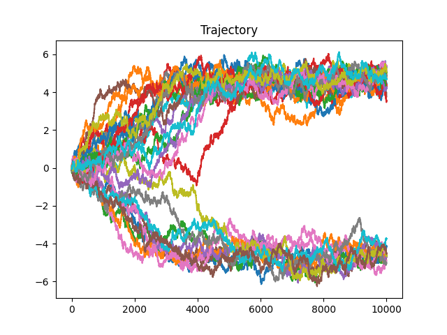
# Plot resulting Trajectories
fig, axs = plt.subplots()
for n, trj in enumerate(data):
    axs.plot(trj["x"])
    axs.set_title("Trajectory")


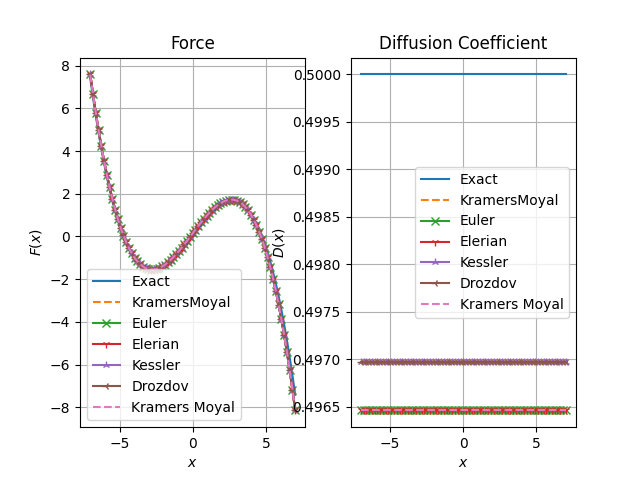
fig, axs = plt.subplots(1, 2)
axs[0].set_title("Force")
axs[0].set_xlabel("$x$")
axs[0].set_ylabel("$F(x)$")
axs[0].grid()

axs[1].set_title("Diffusion Coefficient")
axs[1].set_xlabel("$x$")
axs[1].set_ylabel("$D(x)$")
axs[1].grid()

xfa = np.linspace(-7.0, 7.0, 75)
axs[0].plot(xfa, model_simu.pos_drift(xfa.reshape(-1, 1)), label="Exact")
axs[1].plot(xfa, model_simu.diffusion(xfa.reshape(-1, 1)), label="Exact")
traindrift = fl.functions.Polynomial(deg=3, coefficients=np.array([0, 0, 0, 0]))
trainmodel = fl.models.Overdamped(traindrift, diffusion=fl.functions.Polynomial(deg=0, coefficients=np.asarray([0.9])), has_bias=False)

name = "KramersMoyal"
estimator = fl.KramersMoyalEstimator(trainmodel)
res = estimator.fit_fetch(data)
axs[0].plot(xfa, res.drift(xfa.reshape(-1, 1)), "--", label=name)
axs[1].plot(xfa, res.diffusion(xfa.reshape(-1, 1)), "--", label=name)


for name, marker, transitioncls in zip(
    ["Euler", "Elerian", "Kessler", "Drozdov"],
    ["x", "1", "2", "3"],
    [
        fl.EulerDensity,
        fl.ElerianDensity,
        fl.KesslerDensity,
        fl.DrozdovDensity,
    ],
):
    estimator = fl.LikelihoodEstimator(transitioncls(trainmodel))
    res = estimator.fit_fetch(data)
    # print(res.coefficients)
    axs[0].plot(xfa, res.pos_drift(xfa.reshape(-1, 1)), marker=marker, label=name)
    axs[1].plot(xfa, res.diffusion(xfa.reshape(-1, 1)), marker=marker, label=name)


name = "Kramers Moyal"
res = fl.KramersMoyalEstimator(trainmodel).fit_fetch(data)
axs[0].plot(xfa, res.pos_drift(xfa.reshape(-1, 1)), "--", label=name)
axs[1].plot(xfa, res.diffusion(xfa.reshape(-1, 1)), "--", label=name)


axs[0].legend()
axs[1].legend()

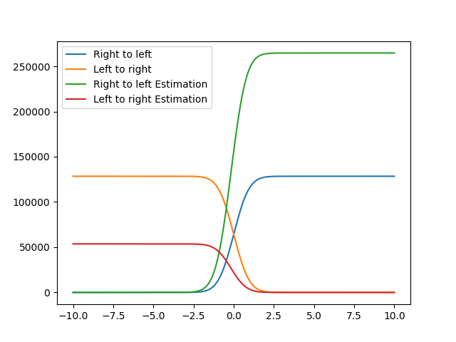
# Compute MFPT from one well to another
plt.figure()

x_mfpt, mfpt = fl.analysis.mfpt_1d(model_simu, -5.0, [-10.0, 10.0], Npoints=500)
plt.plot(x_mfpt, mfpt, label="Right to left")
x_mfpt, mfpt = fl.analysis.mfpt_1d(model_simu, 5.0, [-10.0, 10.0], Npoints=500)
plt.plot(x_mfpt, mfpt, label="Left to right")

x_mfpt, mfpt = fl.analysis.mfpt_1d(res, -5.0, [-10.0, 10.0], Npoints=500)
plt.plot(x_mfpt, mfpt, label="Right to left Estimation")
x_mfpt, mfpt = fl.analysis.mfpt_1d(res, 5.0, [-10.0, 10.0], Npoints=500)
plt.plot(x_mfpt, mfpt, label="Left to right Estimation")
plt.legend()
plt.show()